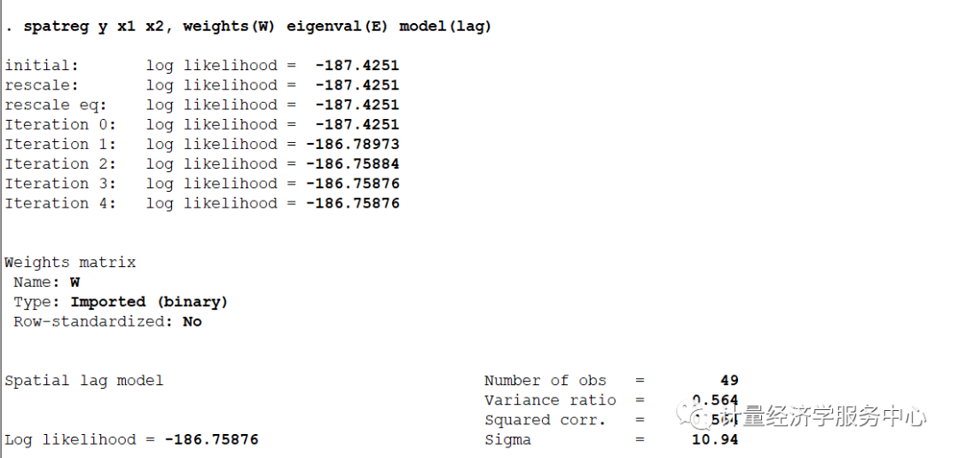
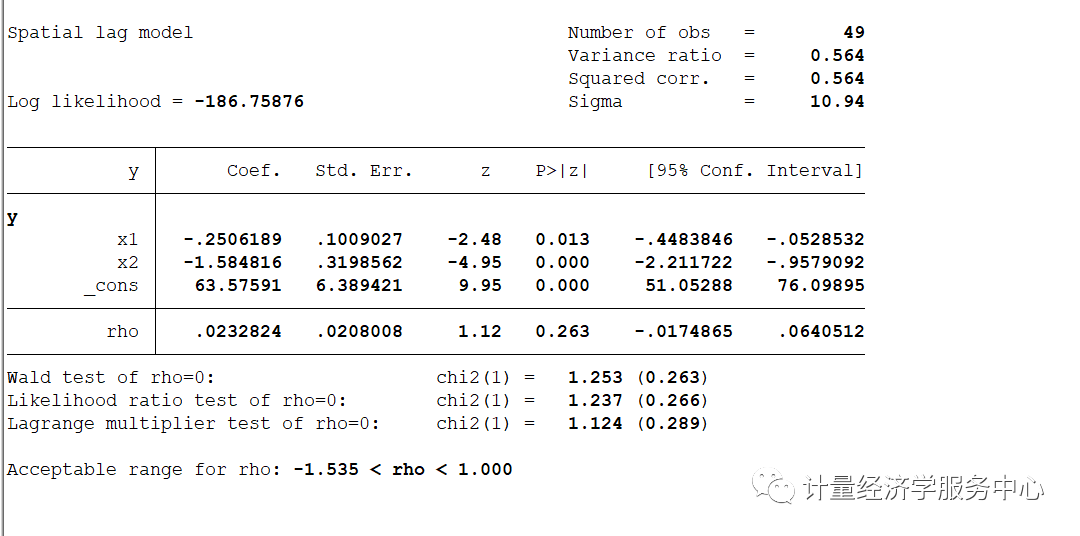
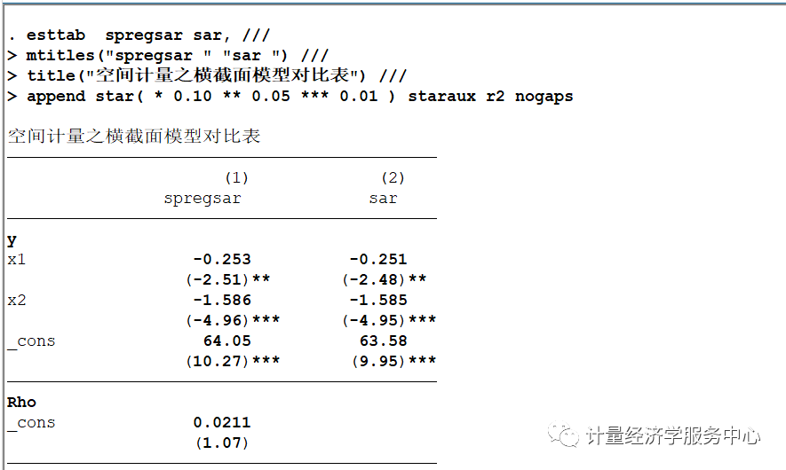
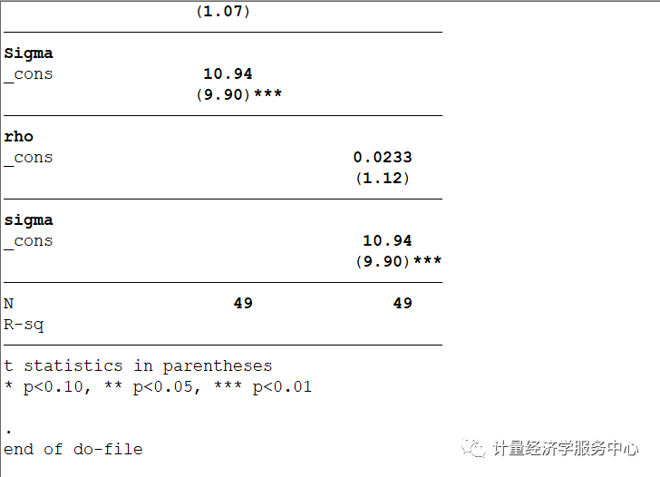
==============================================================================*** Binary (0/1) Weight Matrix: 49x49 (Non Normalized)==============================================================================

initial: log likelihood = -187.4251rescale: log likelihood = -187.4251rescale eq: log likelihood = -187.4251Iteration 0: log likelihood = -187.4251 Iteration 1: log likelihood = -186.83861 Iteration 2: log likelihood = -186.81614 Iteration 3: log likelihood = -186.8161 Iteration 4: log likelihood = -186.8161 ==============================================================================* MLE Spatial Lag Normal Model (SAR)==============================================================================y = x1 + x2------------------------------------------------------------------------------Sample Size = 49Wald Test = 56.4471 | P-Value > Chi2(2) = 0.0000F-Test = 28.2236 | P-Value > F(2 , 47) = 0.0000(Buse 1973) R2 = 0.5510 | Raw Moments R2 = 0.9184(Buse 1973) R2 Adj = 0.5414 | Raw Moments R2 Adj = 0.9166Root MSE (Sigma) = 11.3305 | Log Likelihood Function = -186.8161------------------------------------------------------------------------------- R2h= 0.5510 R2h Adj= 0.5415 F-Test = 28.23 P-Value > F(2 , 47) 0.0000- R2v= 0.5543 R2v Adj= 0.5448 F-Test = 28.61 P-Value > F(2 , 47) 0.0000------------------------------------------------------------------------------y | Coef. Std. Err. z P>|z| [95% Conf. Interval]-------------+----------------------------------------------------------------y |x1 | -.252788 .1007052 -2.51 0.012 -.4501667 -.0554094x2 | -1.585978 .3198759 -4.96 0.000 -2.212924 -.959033_cons | 64.04514 6.233457 10.27 0.000 51.82779 76.26249-------------+----------------------------------------------------------------/Rho | .0211161 .0197638 1.07 0.285 -.0176202 .0598524/Sigma | 10.94111 1.10546 9.90 0.000 8.774445 13.10777------------------------------------------------------------------------------LR Test SAR vs. OLS (Rho=0): 1.1415 P-Value > Chi2(1) 0.2853Acceptable Range for Rho: -0.3199 < Rho < 0.1633------------------------------------------------------------------------------

==============================================================================* Model Selection Diagnostic Criteria==============================================================================- Log Likelihood Function LLF = -186.8161---------------------------------------------------------------------------- Akaike Information Criterion (1974) AIC = 139.1818- Akaike Information Criterion (1973) Log AIC = 4.9358---------------------------------------------------------------------------- Schwarz Criterion (1978) SC = 156.2734- Schwarz Criterion (1978) Log SC = 5.0516---------------------------------------------------------------------------- Amemiya Prediction Criterion (1969) FPE = 136.2414- Hannan-Quinn Criterion (1979) HQ = 145.4344- Rice Criterion (1984) Rice = 140.3238- Shibata Criterion (1981) Shibata = 138.2198- Craven-Wahba Generalized Cross Validation (1979) GCV = 139.7269------------------------------------------------------------------------------

==============================================================================*** Spatial Aautocorrelation Tests==============================================================================Ho: Error has No Spatial AutoCorrelationHa: Error has Spatial AutoCorrelation

- GLOBAL Moran MI = 0.1476 P-Value > Z( 1.984) 0.0472- GLOBAL Geary GC = 0.7581 P-Value > Z(-1.861) 0.0627- GLOBAL Getis-Ords GO = -0.7111 P-Value > Z(-1.980) 0.0476------------------------------------------------------------------------------- Moran MI Error Test = 0.6624 P-Value > Z(8.047) 0.5077------------------------------------------------------------------------------- LM Error (Burridge) = 2.3900 P-Value > Chi2(1) 0.1221- LM Error (Robust) = 2.9300 P-Value > Chi2(1) 0.0869------------------------------------------------------------------------------Ho: Spatial Lagged Dependent Variable has No Spatial AutoCorrelationHa: Spatial Lagged Dependent Variable has Spatial AutoCorrelation

- LM Lag (Anselin) = 0.0097 P-Value > Chi2(1) 0.9215- LM Lag (Robust) = 0.5497 P-Value > Chi2(1) 0.4585------------------------------------------------------------------------------Ho: No General Spatial AutoCorrelationHa: General Spatial AutoCorrelation

- LM SAC (LMErr+LMLag_R) = 2.9397 P-Value > Chi2(2) 0.2300- LM SAC (LMLag+LMErr_R) = 2.9397 P-Value > Chi2(2) 0.2300------------------------------------------------------------------------------

==============================================================================* Heteroscedasticity Tests==============================================================================Ho: Homoscedasticity - Ha: Heteroscedasticity------------------------------------------------------------------------------- Hall-Pagan LM Test: E2 = Yh = 0.9799 P-Value > Chi2(1) 0.3222- Hall-Pagan LM Test: E2 = Yh2 = 0.5735 P-Value > Chi2(1) 0.4489- Hall-Pagan LM Test: E2 = LYh2 = 1.1041 P-Value > Chi2(1) 0.2934------------------------------------------------------------------------------- Harvey LM Test: LogE2 = X = 2.7678 P-Value > Chi2(2) 0.2506- Wald LM Test: LogE2 = X = 6.8293 P-Value > Chi2(1) 0.0090- Glejser LM Test: |E| = X = 7.1015 P-Value > Chi2(2) 0.0287------------------------------------------------------------------------------- Machado-Santos-Silva Test: Ev=Yh Yh2 = 2.8060 P-Value > Chi2(2) 0.2459- Machado-Santos-Silva Test: Ev=X = 7.0429 P-Value > Chi2(2) 0.0296------------------------------------------------------------------------------- White Test -Koenker(R2): E2 = X = 7.1879 P-Value > Chi2(2) 0.0275- White Test -B-P-G (SSR): E2 = X = 9.9225 P-Value > Chi2(2) 0.0070------------------------------------------------------------------------------- White Test -Koenker(R2): E2 = X X2 = 7.5497 P-Value > Chi2(4) 0.1095- White Test -B-P-G (SSR): E2 = X X2 = 10.4218 P-Value > Chi2(4) 0.0339------------------------------------------------------------------------------- White Test -Koenker(R2): E2 = X X2 XX= 18.7572 P-Value > Chi2(5) 0.0021- White Test -B-P-G (SSR): E2 = X X2 XX= 25.8930 P-Value > Chi2(5) 0.0001------------------------------------------------------------------------------- Cook-Weisberg LM Test E2/Sig2 = Yh = 1.3527 P-Value > Chi2(1) 0.2448- Cook-Weisberg LM Test E2/Sig2 = X = 9.9225 P-Value > Chi2(2) 0.0070------------------------------------------------------------------------------*** Single Variable Tests (E2/Sig2):- Cook-Weisberg LM Test: x1 = 0.8877 P-Value > Chi2(1) 0.3461- Cook-Weisberg LM Test: x2 = 4.5468 P-Value > Chi2(1) 0.0330------------------------------------------------------------------------------*** Single Variable Tests:- King LM Test: x1 = 0.0468 P-Value > Chi2(1) 0.8287- King LM Test: x2 = 4.7943 P-Value > Chi2(1) 0.0286------------------------------------------------------------------------------

==============================================================================* Non Normality Tests==============================================================================Ho: Normality - Ha: Non Normality------------------------------------------------------------------------------*** Non Normality Tests:- Jarque-Bera LM Test = 1.6737 P-Value > Chi2(2) 0.4331- White IM Test = 5.4242 P-Value > Chi2(2) 0.0664- Doornik-Hansen LM Test = 3.8663 P-Value > Chi2(2) 0.1447- Geary LM Test = -3.3066 P-Value > Chi2(2) 0.1914- Anderson-Darling Z Test = 0.3147 P > Z( 0.181) 0.5716- D'Agostino-Pearson LM Test = 2.5887 P-Value > Chi2(2) 0.2741------------------------------------------------------------------------------*** Skewness Tests:- Srivastava LM Skewness Test = 0.4911 P-Value > Chi2(1) 0.4835- Small LM Skewness Test = 0.6007 P-Value > Chi2(1) 0.4383- Skewness Z Test = -0.7750 P-Value > Chi2(1) 0.4383------------------------------------------------------------------------------*** Kurtosis Tests:- Srivastava Z Kurtosis Test = 1.0875 P-Value > Z(0,1) 0.2768- Small LM Kurtosis Test = 1.9880 P-Value > Chi2(1) 0.1585- Kurtosis Z Test = 1.4100 P-Value > Chi2(1) 0.1585------------------------------------------------------------------------------Skewness Coefficient = -0.2452 - Standard Deviation = 0.3398Kurtosis Coefficient = 3.7611 - Standard Deviation = 0.6681------------------------------------------------------------------------------Runs Test: (14) Runs - (23) Positives - (26) NegativesStandard Deviation Runs Sig(k) = 3.4501 , Mean Runs E(k) = 25.408295% Conf. Interval [E(k)+/- 1.96* Sig(k)] = (18.6460 , 32.1703 )------------------------------------------------------------------------------

==============================================================================*** Tobit Heteroscedasticity LM Tests==============================================================================Separate LM Tests - Ho: Homoscedasticity- LM Test: x1 = 0.8065 P-Value > Chi2(1) 0.3692- LM Test: x2 = 8.2353 P-Value > Chi2(1) 0.0041

Joint LM Test - Ho: Homoscedasticity- LM Test = 8.2933 P-Value > Chi2(2) 0.0158

==============================================================================*** Tobit Non Normality LM Tests==============================================================================LM Test - Ho: No Skewness- LM Test = 0.4723 P-Value > Chi2(1) 0.4919

LM test - Ho: No Kurtosis- LM Test = 2.5256 P-Value > Chi2(1) 0.1120

LM Test - Ho: Normality (No Kurtosis, No Skewness)- Pagan-Vella LM Test = 2.5809 P-Value > Chi2(2) 0.2751- Chesher-Irish LM Test = 48.9962 P-Value > Chi2(2) 0.0000------------------------------------------------------------------------------

* Beta, Total, Direct, and InDirect (Model= ): Linear: Marginal Effect *

+-------------------------------------------------------------------------------+| Variable | Beta(B) | Total | Direct | InDirect | Mean ||--------------+------------+------------+------------+------------+------------||y | | | | | || x1 | -0.2528 | -0.2522 | -0.2266 | -0.0256 | 38.4362 || x2 | -1.5860 | -1.5824 | -1.4218 | -0.1606 | 14.3749 |+-------------------------------------------------------------------------------+

* Beta, Total, Direct, and InDirect (Model= ): Linear: Elasticity *

+-------------------------------------------------------------------------------+| Variable | Beta(Es) | Total | Direct | InDirect | Mean ||--------------+------------+------------+------------+------------+------------|| x1 | -0.2766 | -0.2760 | -0.2480 | -0.0280 | 38.4362 || x2 | -0.6490 | -0.6475 | -0.5818 | -0.0657 | 14.3749 |+-------------------------------------------------------------------------------+Mean of Dependent Variable = 35.1288

4

操作案例

操作案例2

下面使用上述数据，但是使用spatreg命令进行操作，并对相关结果进行对比

结果对比

可以发现上述结果基本一致